For High Precision Matching, Go Beyond Simple Pairwise Comparisons
How does a researcher connect a patient’s hemoglobin test results with their insulin prescription history with their vital signs measured by wearable technology? Advances in healthcare technology and the accompanying abundance of digital healthcare data can provide researchers with rich views into the holistic patient journey, in this case a patient who may be at risk for diabetes. However, getting to this holistic view is very difficult in today’s real-world data landscape — unless there is confidence that the patients in these datasets can be successfully matched.
Real world datasets are imperfect. They often contain invalid or missing data and patient demographic fields can vary across datasets. Intelligently and accurately stitching together patient records across data sources is therefore paramount for analyses that involve multiple sources of real world data, meet a research-grade standard and require regulatory approval.
The starting point of patient matching is always some form of pairwise matching logic — that is, a criterion that determines whether a pair of records correspond to the same patient. There are a variety of criteria one can use, ranging from deterministic logic such as a rule that links two records if they have the same name and date of birth, to more complex algorithms with probabilistic or machine learning components.
Limitations of pairwise comparisons
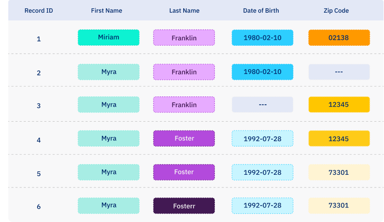
Consider the following table of patient data:

Suppose we use the pairwise comparison rule that two patient records correspond to the same patient if they either:
- Share the same last name, or
- Have at least two demographic fields in common
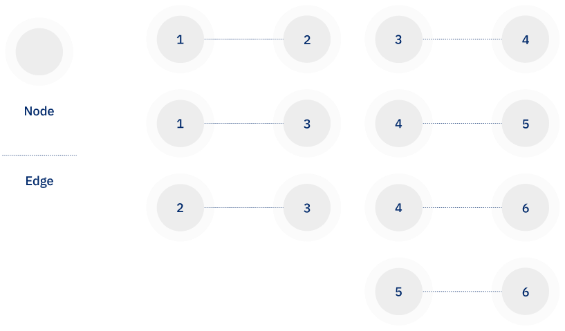
An evaluation of pairs of records in isolation can be represented with pairs of nodes joined by edges, as shown below. The numbers in the nodes correspond to Record IDs in the table, and two nodes are connected if they satisfy the pairwise matching criteria.

This representation suggests that records 1 and 2 should have the same patient ID, as should records 2 and 3. Continuing with this logic suggests that all 6 records should have the same patient ID. The alternative is to make an arbitrary determination as to how to assign patient IDs.
This problem becomes increasingly intractable in real world situations in which we may have hundreds of patient records that are all sequentially connected. Assigning the same patient ID to all such records can result in numerous incorrect patient associations, leading to incorrectly merging patient records and potentially putting patient care at risk. The value of the patient match graph is the added precision achieved by layering it on top of pairwise comparisons.
Advantages of using match graphs
Patient Matching graphs are a data structure that account for multi-record interrelationships by building on pairwise comparisons. Matching algorithms that make use of them boost matching accuracy over approaches that consider each pair of records independently. In particular, the increase in precision is apparent when working with datasets with missing values.
A patient match graph is a representation of patient data that showcases the relationships among patient records. It consists of nodes, with each node representing a single patient record. Two nodes or patient records are connected by an edge if the patient records share enough data to possibly be considered a match; in this way, each edge of the graph represents pairwise comparisons.
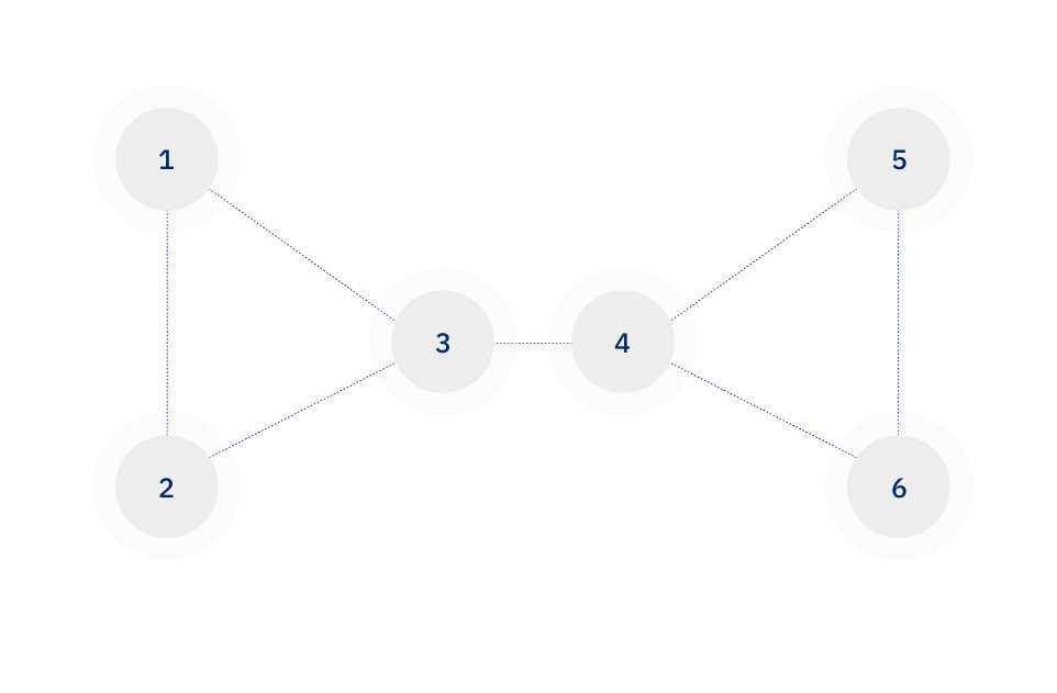
Continuing with our example of the patient records in Table 1, we can use the same criteria for connecting a pair of records that we used when considering pairs in isolation: requiring that a pair of records share either the same last name or at least two demographic fields. This leads to the representation below.

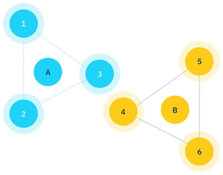
Since we have represented the data as a graph, we can use graph theory to inform our assignment of patient IDs. In the match graph, we can see that there appear to be two clusters of records — one consisting of records 1, 2, and 3, and a second consisting of records 4, 5, and 6. These two clusters are connected by a single “bridge” edge between records 3 and 4. Therefore, we make the decision to cut this bridge edge, and assign patient ID “A” to records 1, 2, and 3, and patient ID “B” to records 4, 5, and 6.

Understanding the complete set of patient interrelationships is a vital piece of assigning accurate patient level IDs. In this example, although 12345 is a real zip code, it could also have been a filler value in this dataset.
Representing the patient records in the form of a match graph enabled a view of the patient population conducive to an algorithm that made the sensible decision of splitting records 1, 2, and 3 from records 4, 5, and 6. Real world data is messier and more complex than our illustrative example, and population level considerations become even more critical for patient matching.
In practice, the manual inspection of the match graph in our example can be implemented in the form of a programmatic algorithm. The result is a means for assigning consistent patient IDs across datasets that is robust in the face of real world data.
Editor’s note: This post has been updated on December 2022 for accuracy and comprehensiveness.


